Background subtraction

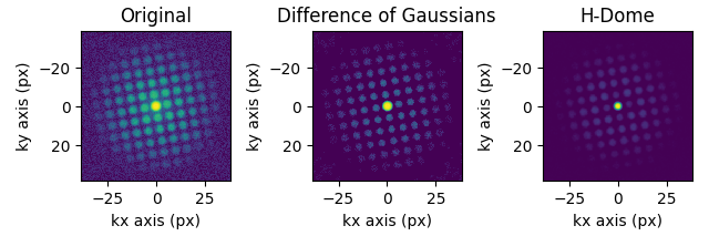
If your diffraction data is noisy, you might want to subtract the background from the dataset. Pyxem offers some built-in functionality for this, with the subtract_diffraction_background class method. Custom filtering is also possible, an example is shown in the ‘Filtering Data’-example.

import pyxem as pxm
import hyperspy.api as hs

s = pxm.data.tilt_boundary_data()

s_filtered = s.subtract_diffraction_background(
    "difference of gaussians",
    inplace=False,
    min_sigma=3,
    max_sigma=20,
)

s_filtered_h = s.subtract_diffraction_background("h-dome", inplace=False, h=0.7)


hs.plot.plot_images(
    [s.inav[2, 2], s_filtered.inav[2, 2], s_filtered_h.inav[2, 2]],
    label=["Original", "Difference of Gaussians", "H-Dome"],
    tight_layout=True,
    norm="symlog",
    cmap="viridis",
    colorbar=None,
)

  0%|          | 0/51 [00:00<?, ?it/s]
 10%|▉         | 5/51 [00:00<00:01, 37.02it/s]
 25%|██▌       | 13/51 [00:00<00:00, 55.45it/s]
 41%|████      | 21/51 [00:00<00:00, 64.62it/s]
 61%|██████    | 31/51 [00:00<00:00, 72.08it/s]
 80%|████████  | 41/51 [00:00<00:00, 73.99it/s]
100%|██████████| 51/51 [00:00<00:00, 75.47it/s]
/opt/hostedtoolcache/Python/3.12.11/x64/lib/python3.12/site-packages/pyxem/utils/_background_subtraction.py:99: FutureWarning: `square` is deprecated since version 0.25 and will be removed in version 0.27. Use `skimage.morphology.footprint_rectangle` instead.
  regional_filter(frame / max_value, **kwargs), footprint=square(3)
/opt/hostedtoolcache/Python/3.12.11/x64/lib/python3.12/site-packages/hyperspy/misc/utils.py:1439: UserWarning: Possible precision loss converting image of type float32 to uint8 as required by rank filters. Convert manually using skimage.util.img_as_ubyte to silence this warning.
  output = function(test_data, **kwargs)

  0%|          | 0/51 [00:00<?, ?it/s]/opt/hostedtoolcache/Python/3.12.11/x64/lib/python3.12/site-packages/pyxem/utils/_background_subtraction.py:99: FutureWarning: `square` is deprecated since version 0.25 and will be removed in version 0.27. Use `skimage.morphology.footprint_rectangle` instead.
  regional_filter(frame / max_value, **kwargs), footprint=square(3)
/opt/hostedtoolcache/Python/3.12.11/x64/lib/python3.12/site-packages/hyperspy/misc/utils.py:1362: UserWarning: Possible precision loss converting image of type float32 to uint8 as required by rank filters. Convert manually using skimage.util.img_as_ubyte to silence this warning.
  output_array[islice] = function(data[islice], **kwargs)

  2%|▏         | 1/51 [00:00<00:09,  5.11it/s]
 10%|▉         | 5/51 [00:00<00:02, 17.98it/s]
 22%|██▏       | 11/51 [00:00<00:01, 30.97it/s]
 29%|██▉       | 15/51 [00:00<00:01, 28.32it/s]
 41%|████      | 21/51 [00:00<00:01, 28.21it/s]
 49%|████▉     | 25/51 [00:00<00:00, 30.56it/s]
 57%|█████▋    | 29/51 [00:01<00:00, 28.89it/s]
 69%|██████▊   | 35/51 [00:01<00:00, 33.31it/s]
 76%|███████▋  | 39/51 [00:01<00:00, 31.01it/s]
 84%|████████▍ | 43/51 [00:01<00:00, 28.90it/s]
100%|██████████| 51/51 [00:01<00:00, 31.73it/s]

[<Axes: title={'center': 'Original'}, xlabel='kx axis (px)', ylabel='ky axis (px)'>, <Axes: title={'center': 'Difference of Gaussians'}, xlabel='kx axis (px)', ylabel='ky axis (px)'>, <Axes: title={'center': 'H-Dome'}, xlabel='kx axis (px)', ylabel='ky axis (px)'>]

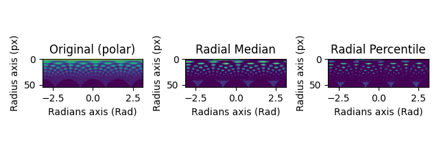
Filtering Polar Images

The available methods differ for Diffraction2D datasets and PolarDiffraction2D datasets.

Set the center of the diffraction pattern to its default, i.e. the middle of the image

s.calibration.center = None

Transform to polar coordinates

s_polar = s.get_azimuthal_integral2d(npt=100, mean=True)

s_polar_filtered = s_polar.subtract_diffraction_background(
    "radial median",
    inplace=False,
)

s_polar_filtered2 = s_polar.subtract_diffraction_background(
    "radial percentile",
    percentile=70,
    inplace=False,
)

hs.plot.plot_images(
    [s_polar.inav[2, 2], s_polar_filtered.inav[2, 2], s_polar_filtered2.inav[2, 2]],
    label=["Original (polar)", "Radial Median", "Radial Percentile"],
    tight_layout=True,
    norm="symlog",
    cmap="viridis",
    colorbar=None,
)

  0%|          | 0/26 [00:00<?, ?it/s]
  4%|▍         | 1/26 [00:03<01:30,  3.62s/it]
 38%|███▊      | 10/26 [00:03<00:04,  3.67it/s]
 81%|████████  | 21/26 [00:03<00:00,  9.04it/s]
100%|██████████| 26/26 [00:03<00:00,  6.71it/s]

  0%|          | 0/51 [00:00<?, ?it/s]
 73%|███████▎  | 37/51 [00:00<00:00, 362.10it/s]
100%|██████████| 51/51 [00:00<00:00, 406.07it/s]

  0%|          | 0/51 [00:00<?, ?it/s]
  2%|▏         | 1/51 [00:00<00:12,  4.05it/s]
 18%|█▊        | 9/51 [00:00<00:02, 19.28it/s]
 33%|███▎      | 17/51 [00:00<00:01, 24.27it/s]
 49%|████▉     | 25/51 [00:01<00:00, 27.42it/s]
 61%|██████    | 31/51 [00:01<00:00, 31.56it/s]
 69%|██████▊   | 35/51 [00:01<00:00, 27.74it/s]
 80%|████████  | 41/51 [00:01<00:00, 28.47it/s]
 92%|█████████▏| 47/51 [00:01<00:00, 32.95it/s]
100%|██████████| 51/51 [00:01<00:00, 29.89it/s]

[<Axes: title={'center': 'Original (polar)'}, xlabel='Radians axis (Rad)', ylabel='Radius axis (px)'>, <Axes: title={'center': 'Radial Median'}, xlabel='Radians axis (Rad)', ylabel='Radius axis (px)'>, <Axes: title={'center': 'Radial Percentile'}, xlabel='Radians axis (Rad)', ylabel='Radius axis (px)'>]